Queueing Systems

Iñaki Ucar

2024-09-28

library(simmer)
library(simmer.plot)
set.seed(1234)

M/M/c/k systems

In Kendall’s notation, an M/M/c/k system has exponential arrivals (M/M/c/k), a $c$ servers (M/M/c/k) with exponential service time (M/M/c/k) and an $k-c$ positions in queue (M/M/c/k). For instance, a router may have several processors to handle packets, and the in/out queues are necessarily finite.

This is the simulation of an M/M/2/3 system (2 server, 1 position in queue). Note that the trajectory is identical to an M/M/1 system (one server, infinite queue).

lambda <- 3
mu <- 4

m.queue <- trajectory() %>%
  seize("server", amount=1) %>%
  timeout(function() rexp(1, mu)) %>%
  release("server", amount=1)

mm23.env <- simmer() %>%
  add_resource("server", capacity=2, queue_size=1) %>%
  add_generator("arrival", m.queue, function() rexp(1, lambda)) %>%
  run(until=2000)

There are rejections when the queue is full.

get_mon_arrivals(mm23.env) %>%
  with(sum(!finished) / length(finished))
#> [1] 0.04253894

By solving the balance equations for this system, we obtain the following:

$$\begin{aligned} p_0 &= \left[ \sum_{n=0}^{c-1}\frac{r^n}{n!} + \sum_{n=c}^{k}\frac{r^n}{c!c^{n-c}} \right]^{-1}\\ N &= \sum_{n=0}^{\infty}nP_n = p_0\left(\sum_{n=0}^{c-n}\frac{nr^n}{n!} + \sum_{n=c}^{k}\frac{nr^n}{c!c^{n-c}}\right) \end{aligned}$$

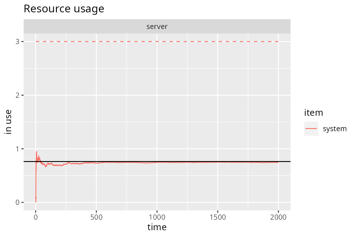
where $r=\lambda/\mu$. Finally, we can see how the simulation quickly converges to the theoretical average number of customers in the system $N$:

# Theoretical value
rho <- lambda/mu
div <- 1 / c(1, 1, factorial(2) * 2^(2:3-2))
mm23.N <- sum(0:3 * rho^(0:3) * div) / sum(rho^(0:3) * div)

# Evolution of the average number of customers in the system
plot(get_mon_resources(mm23.env), "usage", "server", items="system") +
  geom_hline(yintercept=mm23.N)

Custom service policies

Resources implement a FIFO (or FCFS) priority queue, which means that arrivals with a higher priority are processed first, and among those with the same priority, the first-in-first-out policy applies. These priorities can be statically assigned to all arrivals coming from a particular source (using the priority argument in add_generator() or a dedicated column in the data frame passed to add_dataframe()).

However, there is a useful activity to change priorities dynamically (as well as the other two prioritization values, preemtible and restart), and that is set_prioritization(). Such an activity allows us, for example, to implement a LIFO queue just by assigning an increasing priority to incoming arrivals:

env <- simmer()

lifo <- trajectory() %>%
  set_global("resource prio", 1, mod="+") %>%
  set_prioritization(function() c(get_global(env, "resource prio"), NA, NA)) %>%
  seize("resource") %>%
  log_("processing") %>%
  timeout(5) %>%
  release("resource")

env %>%
  add_resource("resource") %>%
  add_generator("dummy", lifo, at(0:4)) %>%
  run() %>% invisible()
#> 0: dummy0: processing
#> 5: dummy4: processing
#> 10: dummy3: processing
#> 15: dummy2: processing
#> 20: dummy1: processing

This mechanism, together with signaling, serves as the basis to implement any custom servicing policy. The main idea is to signal whenever an arrival is going to release the resource so that all the arrivals in the queue can leave the queue momentarily to recompute their priorities:

env <- simmer()

custom <- trajectory() %>%
  renege_if(
    "recompute priority",
    out = trajectory() %>%
      # e.g., increase priority if wait_time < 3
      set_prioritization(function() {
        if (now(env) - get_start_time(env) < 3)
          c(1, NA, NA)     # only change the priority
        else c(NA, NA, NA) # don't change anything
      }, mod="+") %>%
      # go 2 steps back to renege_if
      rollback(2)) %>%
  seize("resource") %>%
  renege_abort() %>%
  log_("processing") %>%
  timeout(5) %>%
  # trigger this before releasing the resource
  send("recompute priority") %>%
  timeout(0) %>%
  release("resource")

env %>%
  add_resource("resource") %>%
  add_generator("dummy", custom, at(0:4)) %>%
  run() %>% invisible()
#> 0: dummy0: processing
#> 5: dummy3: processing
#> 10: dummy4: processing
#> 15: dummy1: processing
#> 20: dummy2: processing

Note that a null timeout was added so that the resource is released in the last place. In this way, all arrivals recompute their priorities and enter the queue again before the resource is released.

State-dependent service rates

In many practical queueing scenarios, the speed of the server depends on the state of the system. Here we consider a multi-server resource that is able to distribute the processing capacity evenly among the arrivals. This means that if, for example, capacity=2 and there is a single arrival in the server, it would be served twice as fast.

In terms of a simulation model, a state-dependent service rate implies that the time spent in the server must be asynchronously updated each time an arrival seizes or releases the resource. In consequence, first we need to define a trajectory that updates a running service delay and restarts the new time left to release the resource. The following trajectory assumes that three attributes are available:

• start: simulation time at which the arrival started the last timeout activity.
• multiplier: distribution of the processing capacity.
• delay: service delay applied to the last timeout activity.

The new delay is the time left scaled by the last and new multipliers.

update.delay <- trajectory() %>%
  set_attribute(c("start", "multiplier", "delay"), function() {
    # previous multiplier, service time left
    multiplier <- get_attribute(env, "multiplier")
    left <- sum(get_attribute(env, c("start", "delay"))) - now(env)
    # distribute processing capacity
    new_multiplier <- capacity / get_server_count(env, "sd.server")
    # return new values
    c(now(env), new_multiplier, left * multiplier / new_multiplier)
  }) %>%
  timeout_from_attribute("delay")

The main trajectory below first seizes the server and initialises the three attributes. Then, the arrivals need to follow the update.delay trajectory and must be interrupted at any given time to re-run it, thus re-computing the service time left. In simmer, this can be done with some signaling (see help(trap)): a signal is subscribed and update.delay is registered as a handler. The first send signals the arriving entity, causing all the arrivals to execute the handler. Eventually, the handler finishes and the execution path returns to unregister the handler, release the server and signal the departing entity.

sd.queue <- trajectory() %>%
  seize("sd.server") %>%
  # initialisation
  set_attribute(c("start", "multiplier", "delay"), function()
    c(now(env), 1, rexp(1, mu))) %>%
  # set the handler
  trap("update delay", handler=update.delay) %>%
  # the following null timeout is required to act as a priority "fence"
  # and get a properly ordered set of simultaneous events
  # (see https://groups.google.com/g/simmer-devel/c/SkOcpu12sT8/m/xG8p5nmTAAAJ)
  timeout(0) %>%
  # trigger the handler
  send("update delay") %>%
  # returning point
  untrap("update delay") %>%
  release("sd.server") %>%
  send("update delay")

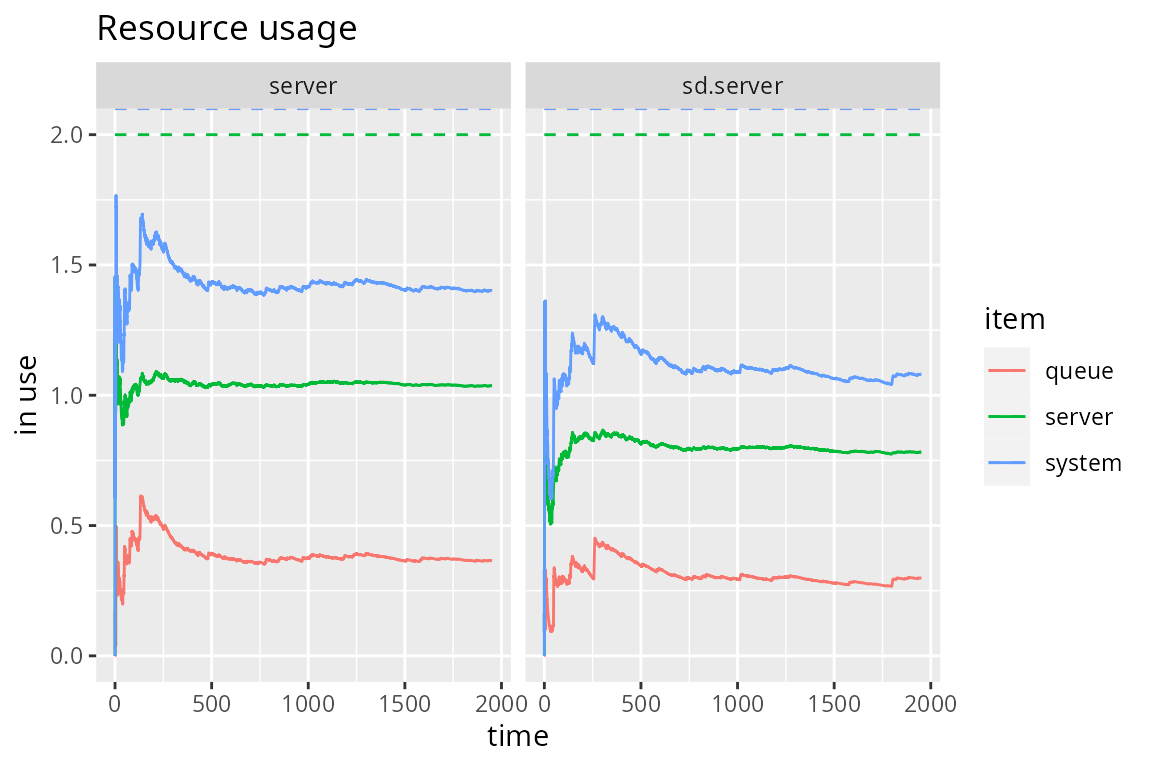
In the following, we compare an M/M/2 with this state-dependent system. Both systems are fed with the same interarrival times and, as expected, the average resource usage is significantly reduced.

lambda <- mu <- 4
capacity <- 2
arrivals <- data.frame(time=rexp(2000*lambda, lambda))

env <- simmer() %>%
  # M/M/2
  add_resource("server", capacity) %>%
  add_dataframe("arrival", m.queue, arrivals) %>%
  # state-dependent service rate
  add_resource("sd.server", capacity) %>%
  add_dataframe("sd.arrival", sd.queue, arrivals)

env %>%
  run() %>%
  get_mon_resources() %>%
  plot(metric="usage", c("server", "sd.server"))

Queueing Networks

Let us consider the following network of queues (example taken from Grotto Networking):

A network of queues.

There are three exponential generators ($\lambda_1$, $\lambda_2$, $\lambda_4$) that inject messages with exponential size of mean 100 bytes. There are four M/D/1 queues with a deterministic rate equal to 220 bytes/s. There is a 25% probability that messages from $\lambda_1$ are dropped before the second queue, and a fork 35/65% for the output of the second queue to reach queues 3 and 4. We are interested, for instance, in the accumulated waiting time for messages entering queue 1 and exiting queue 3 or 4.

We’ll start by setting up the main constants and a couple of functions to set the message size and seize an M/D/1 queue:

mean_pkt_size <- 100        # bytes
lambda1 <- 2                # pkts/s
lambda3 <- 0.5              # pkts/s
lambda4 <- 0.6              # pkts/s
rate <- 2.2 * mean_pkt_size # bytes/s

# set an exponential message size of mean mean_pkt_size
set_msg_size <- function(.)
  set_attribute(., "size", function() rexp(1, 1/mean_pkt_size))

# seize an M/D/1 queue by id; the timeout is function of the message size
md1 <- function(., id)
  seize(., paste0("md1_", id), 1) %>%
  timeout(function() get_attribute(env, "size") / rate) %>%
  release(paste0("md1_", id), 1)

The next step is to set up the three points of attachment for our generators:

to_queue_1 <- trajectory() %>%
  set_msg_size() %>%
  md1(1) %>%
  leave(0.25) %>%
  md1(2) %>%
  branch(
    function() (runif(1) > 0.65) + 1, continue=c(F, F),
    trajectory() %>% md1(3),
    trajectory() %>% md1(4)
  )

to_queue_3 <- trajectory() %>%
  set_msg_size() %>%
  md1(3)

to_queue_4 <- trajectory() %>%
  set_msg_size() %>%
  md1(4)

Finally, we prepare and run the simulation environment with the resources and generators required:

env <- simmer()
for (i in 1:4) env %>% 
  add_resource(paste0("md1_", i))
env %>%
  add_generator("arrival1_", to_queue_1, function() rexp(1, lambda1), mon=2) %>%
  add_generator("arrival3_", to_queue_3, function() rexp(1, lambda3), mon=2) %>%
  add_generator("arrival4_", to_queue_4, function() rexp(1, lambda4), mon=2) %>%
  run(4000)
#> simmer environment: anonymous | now: 4000 | next: 4000.0322040152
#> { Monitor: in memory }
#> { Resource: md1_1 | monitored: TRUE | server status: 1(1) | queue status: 0(Inf) }
#> { Resource: md1_2 | monitored: TRUE | server status: 1(1) | queue status: 3(Inf) }
#> { Resource: md1_3 | monitored: TRUE | server status: 1(1) | queue status: 0(Inf) }
#> { Resource: md1_4 | monitored: TRUE | server status: 0(1) | queue status: 0(Inf) }
#> { Source: arrival1_ | monitored: 2 | n_generated: 8079 }
#> { Source: arrival3_ | monitored: 2 | n_generated: 2044 }
#> { Source: arrival4_ | monitored: 2 | n_generated: 2402 }

In the analysis, we filter arrivals from generator 1 that reach queues 3 and 4, and we examine the average waiting time and the total number of messages:

res <- get_mon_arrivals(env, per_resource = TRUE) %>%
  subset(resource %in% c("md1_3", "md1_4"), select=c("name", "resource"))

arr <- get_mon_arrivals(env) %>%
  transform(waiting_time = end_time - (start_time + activity_time)) %>%
  transform(generator = regmatches(name, regexpr("arrival[[:digit:]]", name))) %>%
  merge(res)

aggregate(waiting_time ~ generator + resource, arr, function(x) sum(x)/length(x))
#>   generator resource waiting_time
#> 1  arrival1    md1_3    5.1816915
#> 2  arrival3    md1_3    0.6969347
#> 3  arrival1    md1_4    4.9417576
#> 4  arrival4    md1_4    0.4751263
get_n_generated(env, "arrival1_") + get_n_generated(env, "arrival4_")
#> [1] 10481
aggregate(waiting_time ~ generator + resource, arr, length)
#>   generator resource waiting_time
#> 1  arrival1    md1_3         3867
#> 2  arrival3    md1_3         2042
#> 3  arrival1    md1_4         2166
#> 4  arrival4    md1_4         2401