Continuous-Time Markov Chains
Iñaki Ucar
2024-09-28
Source:vignettes/simmer-07-ctmc.Rmd
simmer-07-ctmc.Rmd
library(simmer)
library(simmer.plot)
set.seed(1234)
Example 1
A gas station has a single pump and no space for vehicles to wait (if a vehicle arrives and the pump is not available, it leaves). Vehicles arrive to the gas station following a Poisson process with a rate of vehicles per minute, of which 75% are cars and 25% are motorcycles. The refuelling time can be modelled with an exponential random variable with mean 8 minutes for cars and 3 minutes for motorcycles, that is, the services rates are cars and motorcycles per minute respectively.
This problem is described by the following continuous-time Markov chain:
$$\xymatrix{ *=<15mm,8mm>[o][F]{car} \ar@/^/[r]^{\mu_\mathrm{c}} & *=<15mm,8mm>[o][F]{empty} \ar@/^/[l]^{p\lambda} \ar@/^/[r]^{(1-p)\lambda} & *=<15mm,8mm>[o][F]{m/cycle} \ar@/^/[l]^{\mu_\mathrm{m}} }\qquad\qquad Q = \begin{pmatrix} -\mu_\mathrm{c} & \mu_\mathrm{c} & 0 \\ p\lambda & -\lambda & (1-p) \lambda \\ 0 & \mu_\mathrm{m} & -\mu_\mathrm{m} \end{pmatrix}$$
with . The chain is irreducible and recurrent. To theoretically find the steady state distribution, we have to solve the balance equations
with the constraint
There are independent columns, so the latter constraint is equivalent to substitute any column by ones and match it to one at the other side of the equation, that is:
The solution represents the probability of being at each state in the long-term. Therefore, we can calculate the average number of vehicles in the system by summing these probabilities multiplied by the number of vehicles at each state. In our case,
# Arrival rate
lambda <- 3/20
# Service rate (cars, motorcycles)
mu <- c(1/8, 1/3)
# Probability of car
p <- 0.75

# Theoretical resolution
A <- matrix(c(1,   mu[1],            0,
              1, -lambda, (1-p)*lambda,
              1,   mu[2],       -mu[2]), byrow=T, ncol=3)
B <- c(1, 0, 0)
P <- solve(t(A), B)
N_average_theor <- sum(P * c(1, 0, 1)) ; N_average_theor
#> [1] 0.5031056
Now, we are going to simulate the system with simmer and
verify that it converges to the theoretical solution. There are various
options for selecting the model. As a first approach, due to the
properties of Poisson processes, we can break down the problem into two
trajectories (one for each type of vehicle), which differ in their
service time only, and therefore two generators with rates
and
.
option.1 <- function(t) {
  car <- trajectory() %>%
    seize("pump", amount=1) %>%
    timeout(function() rexp(1, mu[1])) %>%
    release("pump", amount=1)

  mcycle <- trajectory() %>%
    seize("pump", amount=1) %>%
    timeout(function() rexp(1, mu[2])) %>%
    release("pump", amount=1)

  simmer() %>%
    add_resource("pump", capacity=1, queue_size=0) %>%
    add_generator("car", car, function() rexp(1, p*lambda)) %>%
    add_generator("mcycle", mcycle, function() rexp(1, (1-p)*lambda)) %>%
    run(until=t)
}
Other arrival processes may not have this property, so we would define a single generator for all kind of vehicles and a single trajectory as follows. In order to distinguish between cars and motorcycles, we could define a branch after seizing the resource to select the proper service time.
option.2 <- function(t) {
  vehicle <- trajectory() %>%
    seize("pump", amount=1) %>%
    branch(function() sample(c(1, 2), 1, prob=c(p, 1-p)), c(T, T),
           trajectory("car") %>%
             timeout(function() rexp(1, mu[1])),
           trajectory("mcycle") %>%
             timeout(function() rexp(1, mu[2]))) %>%
    release("pump", amount=1)

  simmer() %>%
    add_resource("pump", capacity=1, queue_size=0) %>%
    add_generator("vehicle", vehicle, function() rexp(1, lambda)) %>%
    run(until=t)
}
But this option adds an unnecessary overhead since there is an
additional call to an R function to select the branch, and therefore
performance decreases. A much better option is to select the service
time directly inside the timeout function.
option.3 <- function(t) {
  vehicle <- trajectory() %>%
    seize("pump", amount=1) %>%
    timeout(function() {
      if (runif(1) < p) rexp(1, mu[1])  # car
      else rexp(1, mu[2])               # mcycle
    }) %>%
    release("pump", amount=1)

  simmer() %>%
    add_resource("pump", capacity=1, queue_size=0) %>%
    add_generator("vehicle", vehicle, function() rexp(1, lambda)) %>%
    run(until=t)
}
This option.3 is equivalent to option.1 in
terms of performance. But, of course, the three of them lead us to the
same result. For instance,
gas.station <- option.3(5000)

# Evolution + theoretical value
plot(get_mon_resources(gas.station), "usage", "pump", items="system") +
  geom_hline(yintercept=N_average_theor)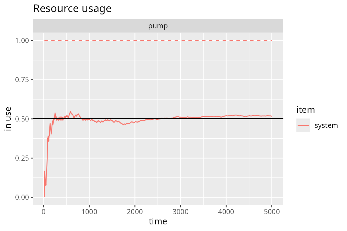
And these are some performance results:
library(microbenchmark)

t <- 1000/lambda
tm <- microbenchmark(option.1(t),
                     option.2(t),
                     option.3(t))
autoplot(tm) +
  scale_y_log10(breaks=function(limits) pretty(limits, 5)) +
  ylab("Time [milliseconds]")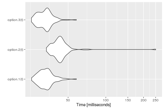
Example 2
Let us complicate things a bit. Consider the previous example, but, this time, there is space for one motorcycle to wait while the pump is being used by another vehicle. In other words, cars see a queue size of 0 and motorcycles see a queue size of 1.
The new Markov chain is the following:
$$\vcenter{\xymatrix{ *=<15mm,8mm>[o][F]{car+} \ar@(r,u)[drr]^{\mu_\mathrm{c}} \\ *=<15mm,8mm>[o][F]{car} \ar@/_/[r]_{\mu_\mathrm{c}} \ar@/^/[u]^{(1-p)\lambda} & *=<15mm,8mm>[o][F]{empty} \ar@/_/[l]_{p\lambda} \ar@/^/[r]^{(1-p)\lambda} & *=<15mm,8mm>[o][F]{m/cycle} \ar@/^/[l]^{\mu_\mathrm{m}} \ar@/_/[d]_{(1-p)\lambda} \\ & & *=<15mm,8mm>[o][F]{m/c+} \ar@/_/[u]_{\mu_\mathrm{m}} }}$$
where the states car+ and m/c+ represent car + waiting motorcycle and motorcycle + waiting motorcycle respectively.
With the steady state distribution, the average number of vehicles in the system is given by
# Theoretical resolution
A <- matrix(c(1,                   0,       0,               mu[1],            0,
              1, -(1-p)*lambda-mu[1],   mu[1],                   0,            0,
              1,            p*lambda, -lambda,        (1-p)*lambda,            0,
              1,                   0,   mu[2], -(1-p)*lambda-mu[2], (1-p)*lambda,
              1,                   0,       0,               mu[2],       -mu[2]),
            byrow=T, ncol=5)
B <- c(1, 0, 0, 0, 0)
P <- solve(t(A), B)
N_average_theor <- sum(P * c(2, 1, 0, 1, 2)) ; N_average_theor
#> [1] 0.6349615
As in the first example, we can simulate this chain by breaking down
the problem into two trajectories (one for each type of vehicle and
service rate) and two generators. But in order to disallow cars to stay
in the pump’s queue, we need to introduce a little trick in the cars’
seize: the argument amount is a function that
returns 1 if the pump is vacant and 2 otherwise. This implies that the
car gets rejected, because there is only one position in queue and that
seize is requesting two positions. Note also that the
environment env must be defined before
running, as it is needed inside the trajectory.
option.1 <- function(t) {
  car <- trajectory() %>%
    seize("pump", amount=function() {
      if (env %>% get_server_count("pump")) 2  # rejection
      else 1                                   # serve
    }) %>%
    timeout(function() rexp(1, mu[1])) %>%
    release("pump", amount=1)

  mcycle <- trajectory() %>%
    seize("pump", amount=1) %>%
    timeout(function() rexp(1, mu[2])) %>%
    release("pump", amount=1)

  env <- simmer() %>%
    add_resource("pump", capacity=1, queue_size=1) %>%
    add_generator("car", car, function() rexp(1, p*lambda)) %>%
    add_generator("mcycle", mcycle, function() rexp(1, (1-p)*lambda))
  env %>% run(until=t)
}
The same idea using a branch, with a single generator and a single trajectory.
option.2 <- function(t) {
  vehicle <- trajectory() %>%
    branch(function() sample(c(1, 2), 1, prob=c(p, 1-p)), c(F, F),
           trajectory("car") %>%
             seize("pump", amount=function() {
               if (env %>% get_server_count("pump")) 2  # rejection
               else 1                                   # serve
             }) %>%
             timeout(function() rexp(1, mu[1])) %>%
             release("pump", amount=1),                 # always 1
           trajectory("mcycle") %>%
             seize("pump", amount=1) %>%
             timeout(function() rexp(1, mu[2])) %>%
             release("pump", amount=1))

  env <- simmer() %>%
    add_resource("pump", capacity=1, queue_size=1) %>%
    add_generator("vehicle", vehicle, function() rexp(1, lambda))
  env %>% run(until=t)
}
We may also avoid messing up things with branches and
subtrajectories. We can decide the type of vehicle and set it as an
attribute of the arrival with set_attribute(). Then, those
attributes can be retrieved using get_attribute(). Although
the branch option is a little bit faster, this one is nicer, because
there are no subtrajectories involved.
option.3 <- function(t) {
  vehicle <- trajectory("car") %>%
    set_attribute("vehicle", function() sample(c(1, 2), 1, prob=c(p, 1-p))) %>%
    seize("pump", amount=function() {
      if (get_attribute(env, "vehicle") == 1 &&
          env %>% get_server_count("pump")) 2    # car rejection
      else 1                                     # serve
    }) %>%
    timeout(function() rexp(1, mu[get_attribute(env, "vehicle")])) %>%
    release("pump", amount=1)                    # always 1

  env <- simmer() %>%
    add_resource("pump", capacity=1, queue_size=1) %>%
    add_generator("vehicle", vehicle, function() rexp(1, lambda))
  env %>% run(until=t)
}
But if performance is a requirement, we can play cleverly with the
resource capacity and the queue size, and with the amounts requested in
each seize, in order to model the problem without checking
the status of the resource. Think about this:
- A resource with
capacity=3andqueue_size=2. - A car always tries to seize
amount=3. - A motorcycle always tries to seize
amount=2.
In these conditions, we have the following possibilities:
- Pump empty.
- One car (3 units) in the server [and optionally one motorcycle (2 units) in the queue].
- One motorcycle (2 units) in the server [and optionally one motorcycle (2 units) in the queue].
Just as expected! So, let’s try:
option.4 <- function(t) {
  vehicle <- trajectory() %>%
    branch(function() sample(c(1, 2), 1, prob=c(p, 1-p)), c(F, F),
           trajectory("car") %>%
             seize("pump", amount=3) %>%
             timeout(function() rexp(1, mu[1])) %>%
             release("pump", amount=3),
           trajectory("mcycle") %>%
             seize("pump", amount=2) %>%
             timeout(function() rexp(1, mu[2])) %>%
             release("pump", amount=2))

  simmer() %>%
    add_resource("pump", capacity=3, queue_size=2) %>%
    add_generator("vehicle", vehicle, function() rexp(1, lambda)) %>%
    run(until=t)
}
We are still wasting time in the branch decision. We can
mix this solution above with the option.1 to gain extra
performance:
option.5 <- function(t) {
  car <- trajectory() %>%
    seize("pump", amount=3) %>%
    timeout(function() rexp(1, mu[1])) %>%
    release("pump", amount=3)

  mcycle <- trajectory() %>%
    seize("pump", amount=2) %>%
    timeout(function() rexp(1, mu[2])) %>%
    release("pump", amount=2)

  simmer() %>%
    add_resource("pump", capacity=3, queue_size=2) %>%
    add_generator("car", car, function() rexp(1, p*lambda)) %>%
    add_generator("mcycle", mcycle, function() rexp(1, (1-p)*lambda)) %>%
    run(until=t)
}
Options 1, 2 and 3 are slower, but they give us the correct numbers, because the parameters (capacity, queue size, amounts) in the model remain unchanged compared to the problem. For instance,
gas.station <- option.1(5000)

# Evolution + theoretical value
plot(get_mon_resources(gas.station), "usage", "pump", items="system") +
  geom_hline(yintercept=N_average_theor)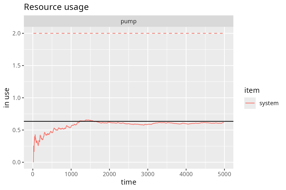
However, it is not the case in options 4 and 5. The parameters of these models are adulterated to fit our performance purposes. Therefore, we need to extract the RAW data, rescale the numbers and plot them. And, of course, we get the same figure:
gas.station <- option.5(5000)

get_mon_resources(gas.station) %>%
  transform(system = round(system * 2/5)) %>% # rescaling
  transform(avg = c(0, cumsum(head(system, -1) * diff(time))) / time) %>%
  ggplot(aes(time, avg)) + geom_line(color="red") + expand_limits(y=0) +
  labs(title="Resource usage: pump", x="time", y="in use") +
  geom_hline(yintercept=2, lty=2, color="red") +
  geom_hline(yintercept=N_average_theor)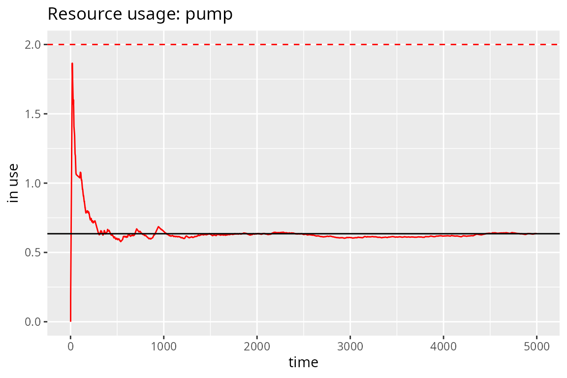
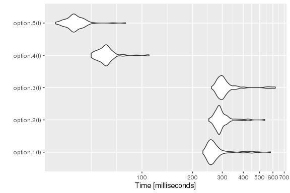
Finally, these are some performance results:
library(microbenchmark)

t <- 1000/lambda
tm <- microbenchmark(option.1(t),
                     option.2(t),
                     option.3(t),
                     option.4(t),
                     option.5(t))
autoplot(tm) +
  scale_y_log10(breaks=function(limits) pretty(limits, 5)) +
  ylab("Time [milliseconds]")